I’m currently developing a survival game using the Unity engine and Blender to create 3D models, along with other programs like Substance Painter for texturing, Photoshop for image edition and Audacity for audio.
The main platform will be Android and the idea is to release a playable prototype on the Play Store in this 2025 year.
In this video I talk about the game project and scope.
#2 – How I work with 3D models
#3 – About random generation items and world objects
In this video I talk about the game project and scope.
Just had this problem, spend hours searching on forums and just found diagnostics but not actual solutions.
If you have an Adobe Software like Photoshop or if you have a friend that has it, you can get the LIBEAY32.dll file in a safe way, without having to download it from a website that you don’t know if you can trust.
Video showing the way I solved the problem:
You have reach the end of the article, if it was useful consider subscribing to the channel!
Using GitHub you can have your projects backed up on the cloud, collaborate with others or just access to your projects from different computers.
In this article we will see how to use GitHub desktop to clone a Unity project from a GitHub repository, it’s a super easy process that doesn’t require you to learn console commands, just make a few clicks on GitHub Desktop. When you clone a Unity project from GitHub you get the project files in the location you indicate, so you will also need to add that project in Unity HUB.
Then you need to download GitHub Desktop, a software that allows you to easily work with Git without using console commands, which could be difficult to set up and learn how to use. With GitHub Desktop you will be able to perform most of basic Git operations and it’s a nice way to start.
Install GitHub desktop and log into the account created in the first step.
Find the link of a Unity project repository you want to clone. Here you have two of my repositories for testing:
GDT Solutions for Unity
In this repository you will find a collection of solutions like a drag-and-drop first person controller or how to change from one scene to another in Unity.
The Unity project files of a mini game where you have to find a set of objects randombly hide inside a maze in order to get the key that opens the gate to escape from the maze.
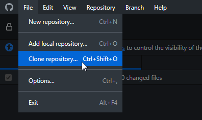
Inside GitHub Desktop go to File > Clone Repository, select the URL tab and paste the link of the GitHub repository you want to clone.
Choose a folder where you want to store the project files, in my case I have a Unity folder where I have all my projects and I would use that folder because we are cloning a Unity repository, but you could choose any folder you want.
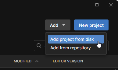
After the process is finished, we already have the files in the location we indicate and as you can see these files correspond to a Unity project, so for the next step let’s open Unity HUB and add a project from disk.
Select the folder of the project and press Add Project, so now you already have the project in your Unity HUB and you can open it to check the solutions.
How to keep a repository updated
I will be adding more solutions to the GDT Solutions for Unity repository and also keep this project updated with the latest Unity’s LTS version. So if you want to receive new solutions make sure to follow my GitHub account and also watch the repository.
To look for new updates go to GitHub desktop, make sure you are in the right repository, discard all unnecesary changes, click here to refresh and if a new Update is available just press “Pull” and wait to the process is finished.
Then go back to Unity and reload the scene if necesary, that way you could receive new solutions that I will be making from time to time.
You have reach the end of the article, if it was useful consider subscribing to the channel!
First of all, you don’t need to export the 3D model in Blender because you can perfectly work in Unity using the Blender files, you just need to take the blend file and all the textures aplied to the model, move all the files to a folder inside your project in Unity and then you can take the Blend file and drag it to the scene in Unity, doing that you can use the Blender models in Unity.
The textures of the 3D model could not be automatically applied when you do the previous step, so we will see how to apply the textures to the 3D model that was exported from Blender, but first let me suggest to check the following video in which I explain all the process in detail:
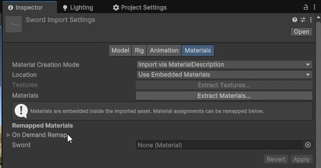
In your Unity project select the blend file and in the inspector go to the Materials section (leave the image for reference) and there you will find all the materials that you defined in Blender, to remap the materials you have two options, you either replace the materials from the 3D model with new materials created in Unity or you extract the materials present in the Blend file.
Remap the Blender materials with new materials created in Unity
Create a new material.
Drag the material to the material field in the inspector.
Click on apply to remap.
Drag the textures to the material and adjust parameters to get the result you need.
Repeat the previous steps for every material your model has.
Remap the Blender materials by extracting them from the 3D model
Unfold the Blend file to find all the materials defined in Blender.
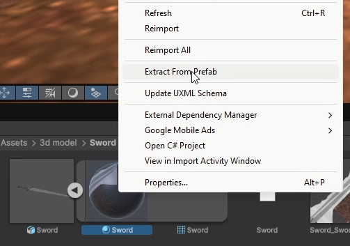
Select all the materials, right click and choose “extract from prefab” (check image below).
Save those materials and that way Unity create all the materials for you and automatically remap to those materials.
Drag the textures to the material and adjust parameters to get the result you need.
You have reach the end of the article, if it was useful consider subscribing to the channel!
The purpouse of this entry is to show a very simple example of application in Unity, an electrical circuit with a DC source connected to a resistor.
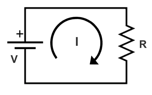
The DC source provides a constant voltage over time and the resistor is a passive electrical component that is characterized by offering resistance to the flow of electric current. When these two components are connected as shown in Figure 1, a current is established that will be proportional to the voltage and inversely proportional to the resistance, according to Ohm’s Law:
I = V / R
Fig.1: Electrical circuit with DC source and a resistor, the current flowing will be calculated by applying Ohm’s Law.
Screenshots of the program running
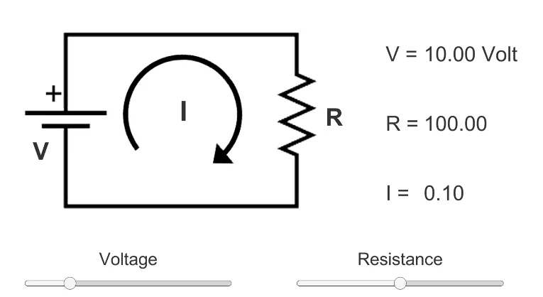
Figures 2 and 3 show the program running, the circuit diagram is a representative image, the three values on the right are the actual values of the system, the voltage and resistance are variable parameters that can be changed using the sliders at the bottom and the current is calculated as a result of these values.
Fig. 2: Screenshot of the program running, the sliders allow to modify the voltage and resistance values, the current is calculated by applying Ohm’s Law.
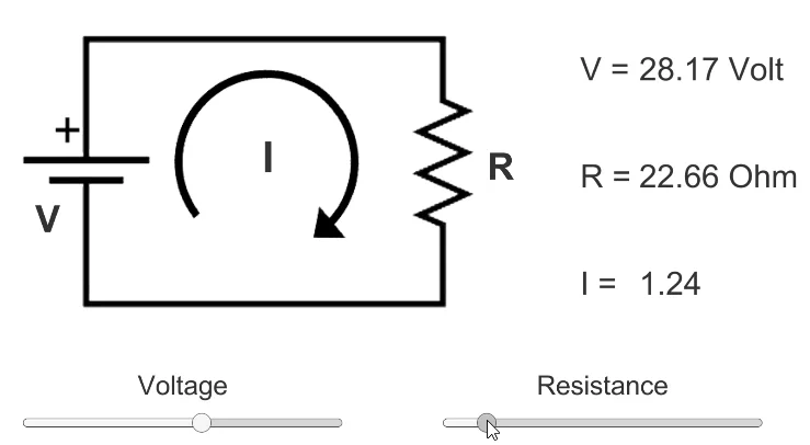
Fig. 3: Another snapshot of the program with other values.
Analysis of the Script that controls the system
The script responsible for controlling the system and displaying the information on the screen is analyzed below.
Then, three float variables are defined for the voltage, resistance and current of the circuit (lines 13, 14 and 15).
Fig. 4: Script variables controlling the DC circuit simulator.
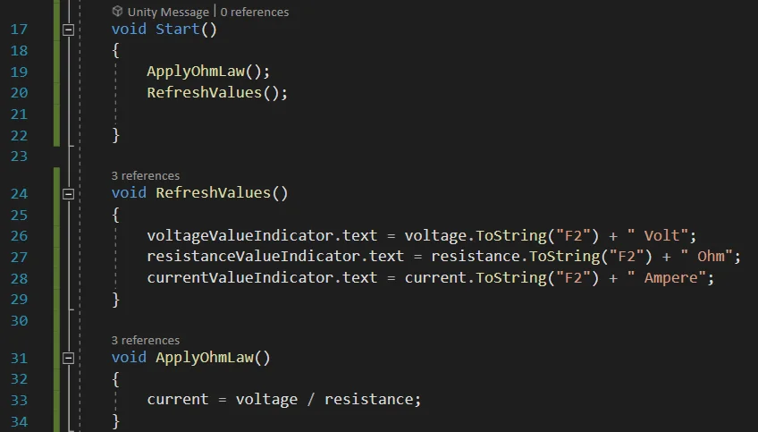
Start function, value update on the screen and Ohm’s Law calculation
In figure 5 there are three functions belonging to the system. Start is a function that Unity executes automatically after pressing the Play button and before the first frame of the application is displayed, within this function Ohm’s Law is applied with the initial values that are defined and the values are refreshed on screen, this occurs in the execution of the methods of lines 19 and 20 respectively.
The “RefreshValues” method is responsible for writing the voltage, resistance and current values to the Text components of the graphical interface.
The “ApplyOhmLaw” method performs the calculation of the current as a function of the voltage and the resistance, here you could have an indeterminacy if the resistance (the denominator) is null, if this happens there is no error at run time, but Unity detects this situation and solves it by assigning the value “Infinity”, which serves as an indicator that there is an indeterminacy.
Fig. 5: Script functions controlling the DC circuit simulator, initialization, Ohm’s Law and GUI update.
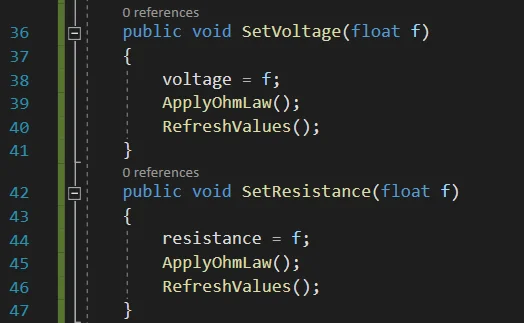
Functions for modifying values from the graphical interface
In order for the Sliders of the graphic interface to be able to modify values within a Script, they must do it through public methods, the methods shown in figure 6 fulfill this purpose, the top one allows to modify the voltage value and the bottom one the resistance value. Note that not only the values are modified but also Ohm’s Law is recalculated and the values are refreshed on the screen.
Fig. 6: Functions of the script that controls the DC circuit simulator, public methods that allow to modify the voltage and resistance values by manipulating the sliders of the graphical interface.
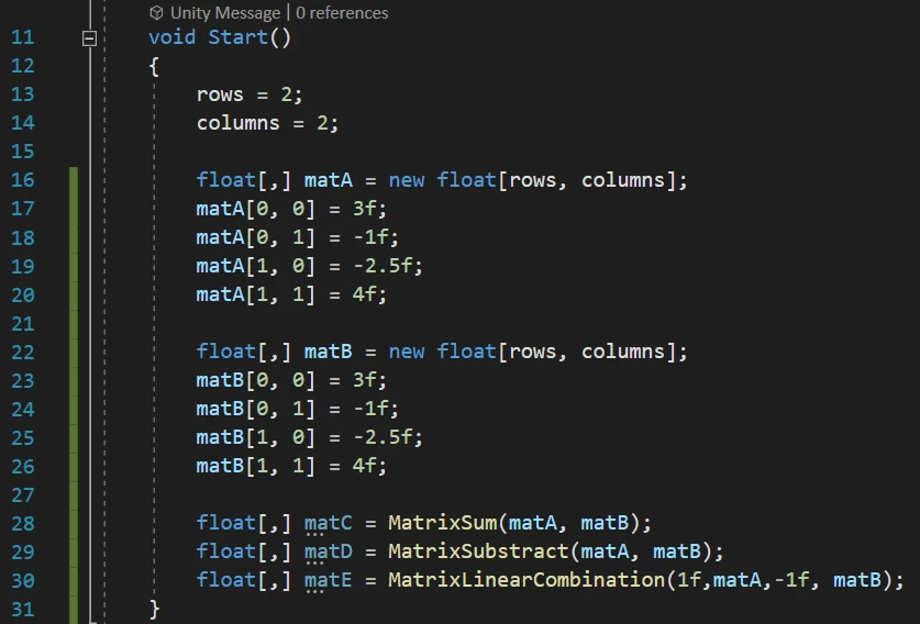
We will start from two matrices “A” and “B” with preloaded data and we will analyze a method that will multiply two matrices that are sent as parameter and returns the result matrix.
In figure 1 we see the declaration of two 2×2 matrices and the loading of their data, then in lines 27 and 28 we make the calls to the method that is in charge of multiplying the matrices that are sent as parameters and returning the resulting matrix.
Fig. 1: Declaration of two matrices A and B, data loading and execution of the function that multiplies two matrices passed as parameters.
Algorithm for multiplying matrices in programming
The product of matrices is not commutative, so it matters the order in which the matrices are multiplied. Let’s consider that matrix A is on the left and multiply it by matrix B which is on the right.
The procedure to multiply two matrices consists of multiplying each element of the i-th row of the left matrix by each element of the j-th column of the right matrix and then adding these products, the result of that sum will be the ij-element of the resulting matrix. Therefore, in order to carry out the product of matrices, the condition that the number of columns of the left matrix equals to the number of rows of the right matrix must be fulfilled.
The result of the multiplication of matrices A and B will be another matrix that will have a number of rows equal to the number of rows in A and a number of columns equal to the number of columns in B.
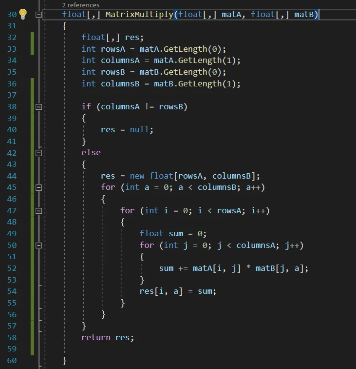
Algorithm analysis
Figure 2 shows the implementation of an algorithm that multiplies two matrices that are sent as parameters. First the result matrix is declared and the sizes of both matrices are read, this is done in lines 32 to 36.
Then we check if it is possible to multiply both matrices, if it is not possible the result will be null, otherwise we proceed to solve the product of matrices.
The resulting matrix structure is created with the corresponding number of rows and columns (see the description of the procedure above). Then the three nested for loops shown in figure 2 are used to determine the value of each resulting element.
Fig. 2: Algorithm that solves the multiplication of two matrices received as parameters and returns a matrix that is the result of the product of both matrices.
To be able to add or subtract two matrices it is necessary that both have the same size, that is to say the same number of rows and the same number of columns, otherwise the operation cannot be solved. We will take this into account in our algorithm, at the time of performing the operation we will check that these conditions are met and if everything is correct the sum will be solved, otherwise the returned matrix will have a null value and this result can be used to make subsequent checks, for example if the resulting matrix is different from null we consider that the operation was successful.
Initial data
We will start from two matrices “A” and “B” with preloaded data and we will analyze a method that will perform the sum of two matrices that are sent as parameter and returns the result matrix.
In figure 1 we see the declaration of two 2×2 matrices and the loading of their data, then in lines 28, 29 and 30 we make the calls to the methods that will be in charge of adding, subtracting or making a linear combination between the matrices that are sent as parameter, those methods will return the resulting matrix.
Fig. 1: Declaration of two matrices A and B, data loading and execution of the methods that add, subtract and perform a linear combination of both matrices.
Algorithm to add two arrays in programming, C# language
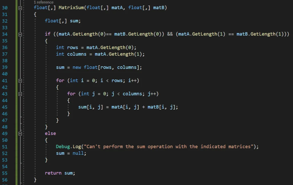
To make the sum of two matrices we must first make sure that both matrices have the same size, if this is correct we proceed to go through each element of the matrices and perform the sum element by element, assigning the result to a new matrix previously declared.
Fig. 2: Algoritmo para sumar dos matrices A y B implementado en lenguaje C#, ejemplo en Unity.
Analysis of the algorithm that performs the addition of two matrices
Between lines 30 and 56 we have defined a method that receives as parameters two two-dimensional arrays (“matA” and “matB”) and returns another two-dimensional array.
The result matrix is declared on line 32 and returned on line 55, at the end of the procedure.
Then in line 34 we have an IF statement to check if it is possible to solve the sum of the matrices, the condition is that the matrices match in number of rows and columns, if this is true we proceed to solve the sum, otherwise a message is printed on the console indicating that it is not possible to solve the operation and the result variable is assigned null (lines 51 and 52).
If the sum of matrices can be solved we will determine the number of rows and columns of the result matrix and we will create the data structure for that matrix, we do this in lines 36, 37 and 39 respectively.
The addition of the matrices is done element by element, therefore we will use two nested loops, the first one will go through each row and the inner loop will go through each column, so we will start with a row and go through each of the columns, at the end we will go to the next row. Inside the inner loop we simply solve the sum of the ij-elements of each matrix and assign it to the ij-element of the result matrix.
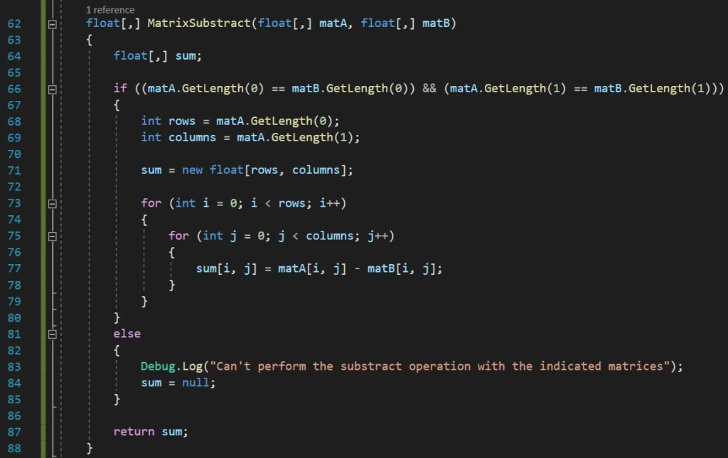
Algorithm to subtract two matrices in programming, C# language
To subtract two matrices in programming, the algorithm is practically the same as the addition, only that when their elements are traversed, instead of adding them, they are subtracted, we can see an implementation of the algorithm in Figure 3.
Fig. 3: Algorithm to subtract two matrices A and B implemented in C# language, example in Unity.
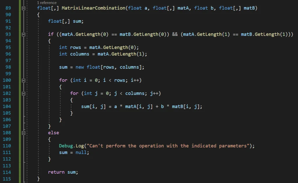
Algorithm to perform the linear combination of two matrices in programming, C# language.
Since the algorithms for adding and subtracting matrices are very similar, a function could be defined that performs a linear combination between the two matrices indicated together with their coefficients, i.e. it solves the operation:
MatrixC = a * MatrixA + b * MatrixB
In this way to perform the subtraction of matrix A minus matrix B we could call this function passing as parameter 1 for the coefficient that multiplies matrix A and -1 for the coefficient that multiplies matrix B, but we also have a function with higher capabilities. In Figure 4 we see the algorithm that solves the linear combination between both matrices.
Fig. 4: Algorithm to solve the linear combination of two matrices A and B implemented in C# language, example in Unity.
We will start from an “A” matrix with preloaded data and we will analyze a method that will perform the transposition of the matrix sent as parameter and will return the result matrix.
Fig. 1: Declaration of a matrix “A” and call to a function that returns its transposed matrix.
Algorithm for transposing matrix of N rows and M columns
Transpose a matrix implies transforming its rows into columns and its columns into rows, therefore the resulting matrix will be a matrix that will have its dimensions exchanged. The function that will be in charge of transposing the matrix that enters as parameter is shown in figure 2, first we will read the number of rows and columns of the input matrix and we will create the structure of the result matrix, this is done in lines 30, 31 and 32 respectively, notice how in the creation of the result matrix, the dimension is exchanged comparing with the input matrix.
Then we have to traverse each element of the input matrix, we have seen that this could be done by two nested for-loops, the first one traverses rows and the inner loop traverses columns. Inside the loop what we will do is to assign the ij-element of the input matrix, to the ji-element of the output matrix.
At the end of the loop, the result matrix is returned (line 41).
Fig. 2: Algorithm for transposing a matrix.
Introduction
In mathematics, a matrix is a structure containing numerical data arranged in rows and columns, one of its main uses is to represent and solve systems of linear equation.
In this article you will see how to represent a matrix and load data to it in C# language in Unity Engine.
About the development environment, script creation and execution
For this example we will use the Unity engine, create a C# Script and assign it to a GameObject in the scene, when pressing the Play button, Unity will automatically execute some functions inside the Script.
Implementation of a matrix in programming
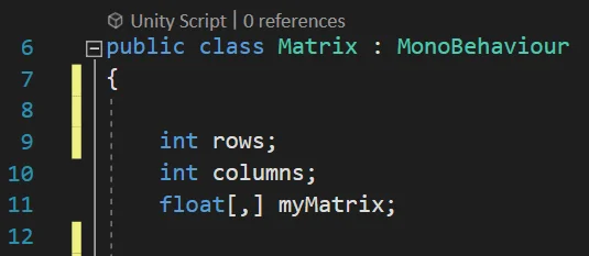
Declaration of data
Matrices have a certain number of rows and columns, so we will need two integers, let’s call them “rows” and “columns”.
To declare the matrix in programming we will use a two-dimensional arrays and we must indicate the data type, usually we are going to work with the set of real numbers, so the data type we are going to use is “float”. However we could define arrays of any data type needed, for example “bool”, “int”, “double”, “string”, etc.
The declaration of the required data would be as follows:
Fig. 1: Data declaration to represent a matrix size “rows” by “columns”.
To declare a two-dimensional array, brackets are used and a comma is placed for each extra dimension that is needed, in this case as we need two dimensions it looks like this: “[ , ]”.
Initialization of the matrix data
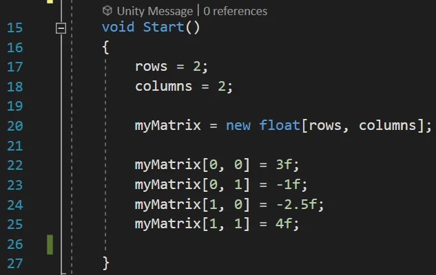
In the previous step we declared the necessary variables, now it is time to initialize those variables, that is to say to give them concrete values or to create data structures and assign them. The initialization will be done in the “Start” method of the Script, the Start and Update functions are automatically defined when creating a new Script. By pressing the Play button in Unity, the Start functions of all the scripts present in the scene will be automatically executed, this will happen before the the first frame of the program appears on the screen.
In figure 2 we see an example of the initialization of a 2×2 matrix, in lines 17 and 18 is the initialization of the rows and columns respectively. In line 20 a two-dimensional array is created indicating the total number of elements of each dimension and this array is assigned to the “myMatrix” field that was declared in the previous step.
Fig. 2: Inicialización de los datos necesarios para representar una matriz de 2 filas y 2 columnas.
In C# the first element of the arrays is 0 and the last is “n-1”, where n is the size of the array, so in line 22 for example, the data in position [0,0] refers to the element in the first row and first column.
Conclusion
We have seen how to declare two-dimensional arrays that can be used to represent matrices and subsequently perform operations between them.
In this example the data type used for the array is “float”, which means that each element will have a number with decimal point stored, but you could define arrays of any data type you need, for example “bool”, “int”, “double”, “string”.
To read or modify an element within the matrix we use the name with which it was defined and between brackets we indicate the row and column separated by comma, so for example if we write “myMatrix[1,0]” we are pointing to the element of the matrix that is in the second row, first column.
Introduction
A resistive voltage divider is an arrangement of two resistances in series that allows us to have at the midpoint a fraction of the voltage at the ends.
Applications of a resistive divider
The divider with potentiometer is usually used as an analog input in the frequency driver of the motors. Using the potentiometer we change the speed of the motor.
A BJT transistor can also be polarized with a splitter, connecting the central point of the splitter to the base of the transistor.
Working principle of the resistive divider
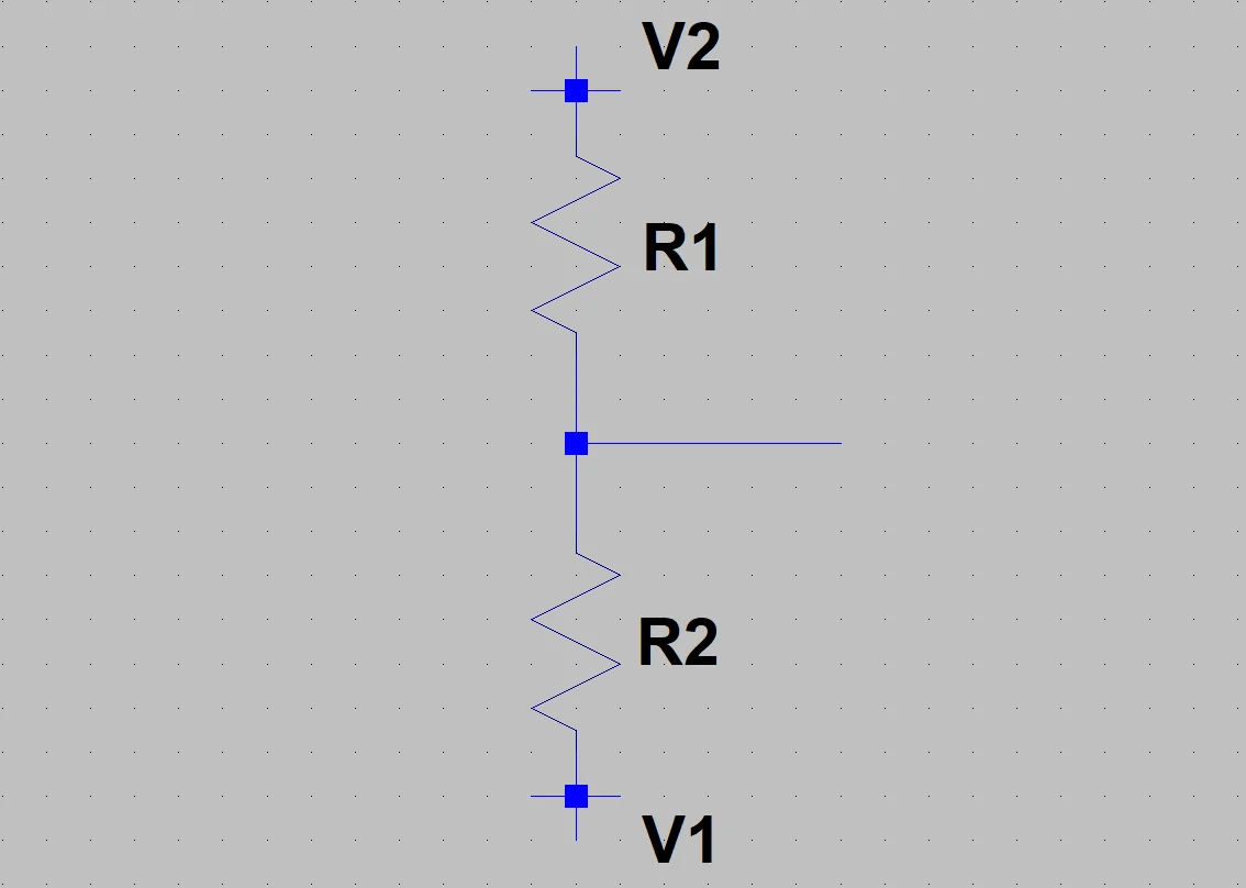
In figure 1 we see an arrangement that can be used as a divisor.
Fig. 1: Generic resistive divider in LT Spice.
To understand how it works we must consider the potential drops in both resistances.
The voltage drop on a resistor is the current flowing through it multiplied by the resistive value.
We are going to analyze two cases, when the resistances are equal and when one is greater or less than the other.
Case 1: Equal Resistors
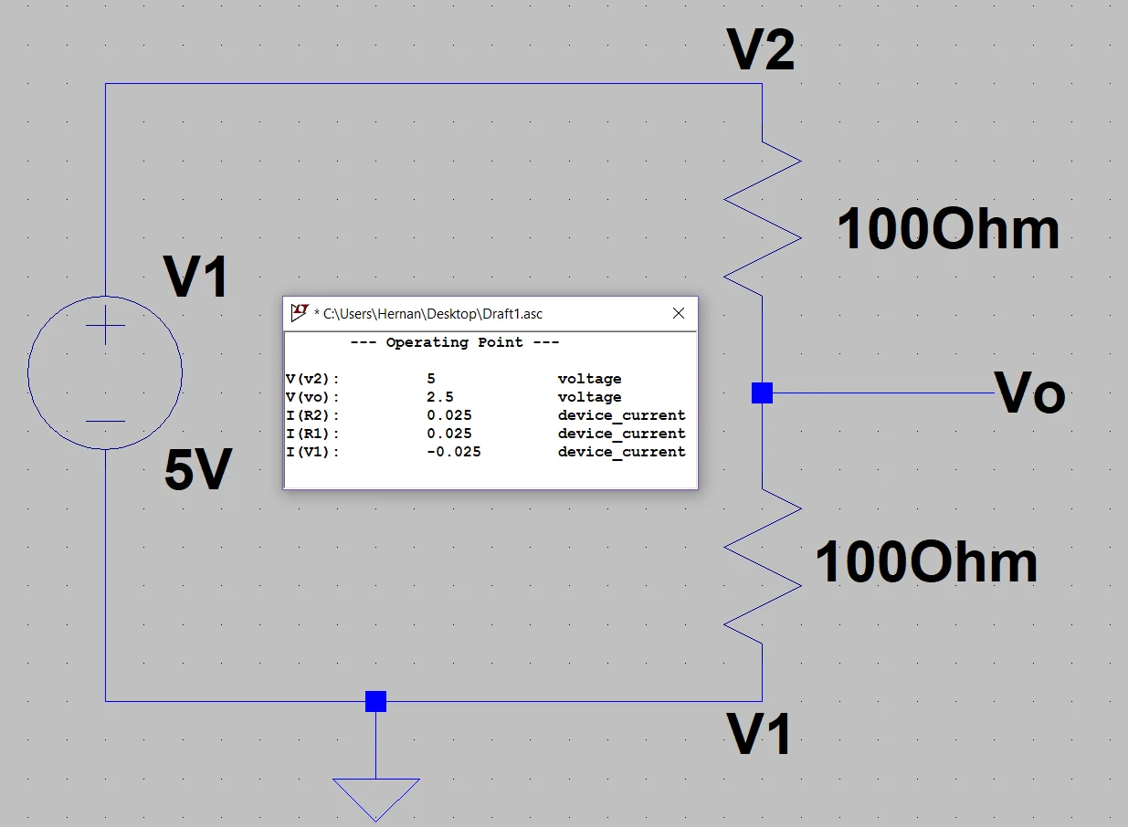
In this case we can intuit that the potential drop in both resistances will be the same (because the same current circulates through them and their resistive value is equal), therefore at the midpoint of the divisor we will have a voltage value equal to the mean value between the potential difference at the extremes.
In figure 2 we can see that the voltage in Vo is 2.5 Volts, half of the 5 Volts applied in the divisor.
With this result we may be tempted to say that the voltage at the midpoint of the divisor is going to be equal to half the value applied in V2, but this is not always the case.
This is only fulfilled if in V1 we have applied 0 Volts (in figure 2 V1 is grounded).
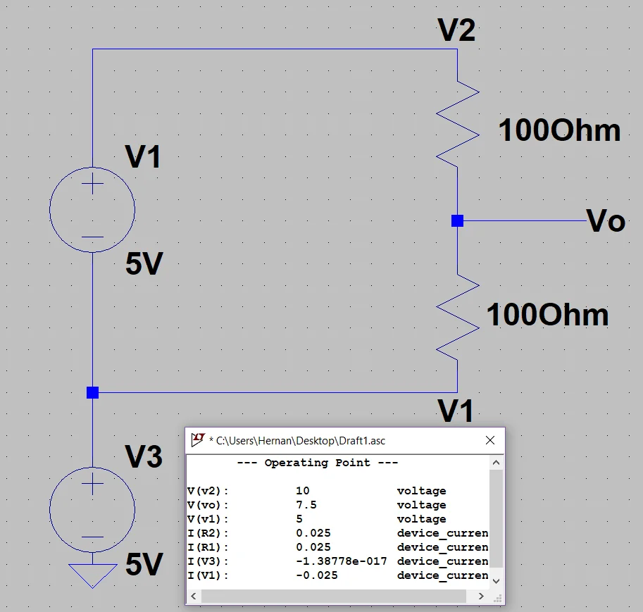
In figure 3 we see an example in which this is not fulfilled, in this case the potential difference in the divisor is still 5 Volts, but V1 is not grounded but has applied 5 Volts while V2 has 10 Volts.
The result is that in Vo we have half the applied potential difference plus the voltage V1.
Fig. 2: The voltage at the midpoint of the divisor is equal to half of the applied voltage.
Fig. 3: Voltage at Vo does not match half of the applied potential difference at the ends.
Case 2: Different Resistors
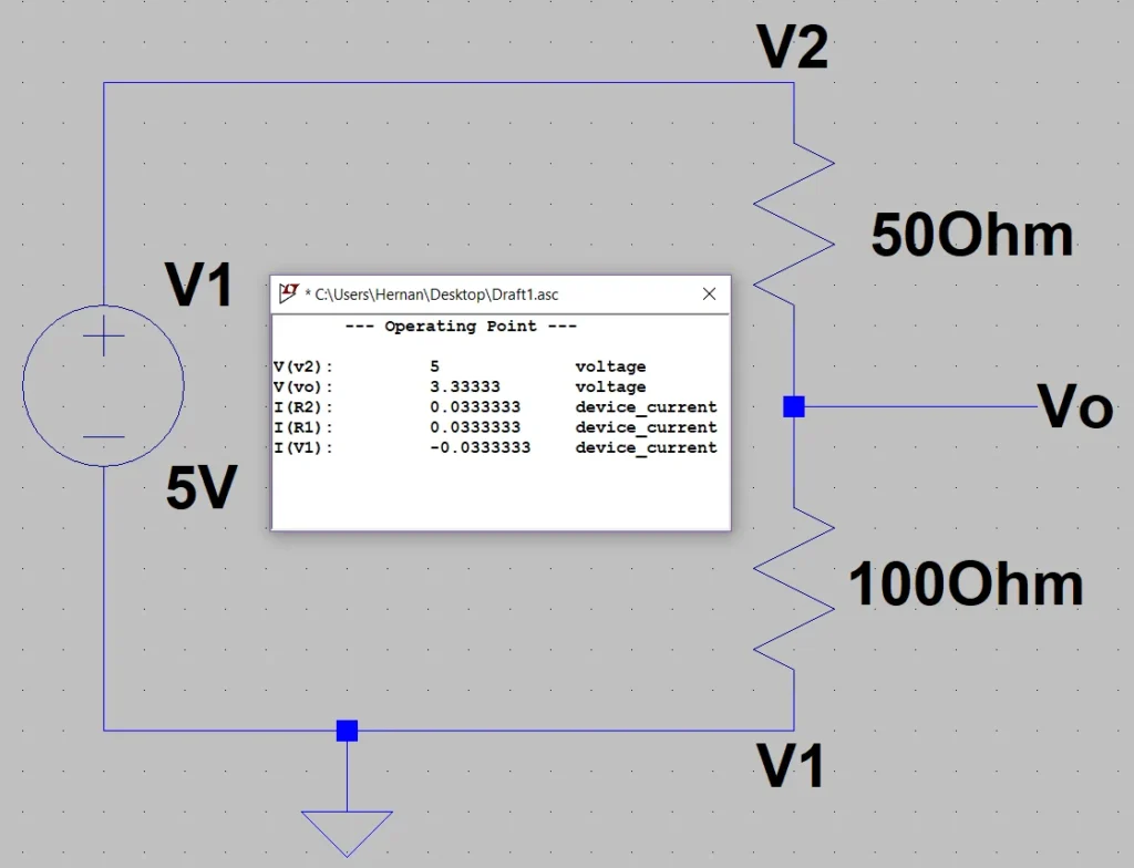
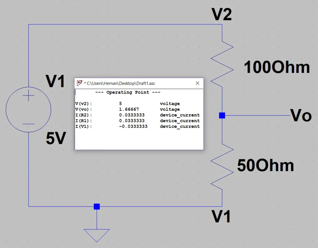
In figure 4 we consider R1 smaller than R2 and in figure 5 the opposite case.
Fig. 4: The voltage at Vo is greater than half the difference in potential applied at the ends.
Fig. 5: The voltage at Vo is less than half the potential difference applied at the ends.
Based on the results we can say that if 100% of the resistive value is 150 Ohms, 50 Ohms and 100 Ohms will be approximately 33% and 66% respectively.
These percentages seem to be reflected in the Vo voltage, as in Figure 4 the 3.3 V voltage is approximately 66% of 5 V while 1.6 V is approximately 33% of 5V.
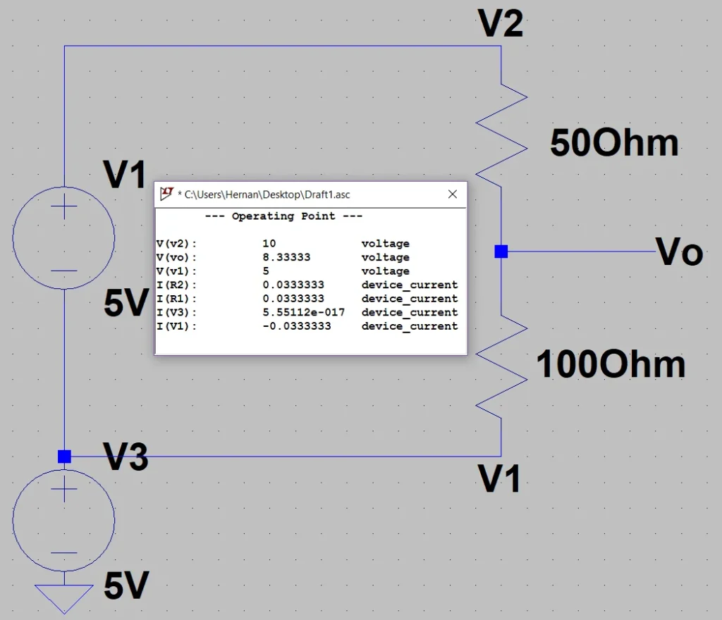
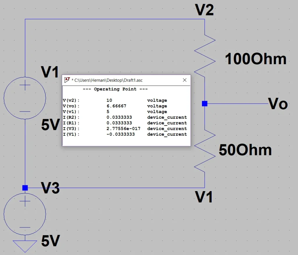
Analogously to figure 3, we should not assume that this will always be so, we must remember to add the voltage applied in V1, we can see this in figures 6 and 7.
Fig. 6: The result in figure 4 must be added to the voltage applied in V1.
Fig. 7: The result of figure 5 must be added to the voltage applied in V1.
Formula deduction
Now that we have seen the working principle and some experiments we are going to find an expression for the voltage Vo that takes into account both resistances.
The voltage Vo will be equal to the voltage V1 plus the potential drop in resistance 2.
Vo = V1 + Vr2
The potential drop in R2 is equal to the current flowing through the resistance multiplied by the value of R2.
Vr2 = i x R2
Then:
Vo = V1 + i x R2
The current circulating through the divisor, by Ohm’s Law, is equal to the difference of potential applied at the ends divided by the sum of the resistances.
i = ( V2 – V1 ) / ( R1 + R2 )
Replacing the current in the previous expression we have:
Vo = V1 + R2 x ( V2 – V1 ) / ( R1 + R2 )
Here we already have an expression for Vo in which are all the variables of figure 1, however we can solve the sum and obtain a more compact expression.
Vo = ( R1 x V1 + R2 x V2) / ( R1 + R2 )
The Potentiometer
This element can be used as a variable resistive divider.
The potentiometer is basically two resistors that we can change value but the sum of both remains unchanged.
If we connect a potential difference at the ends, in the middle we will have a voltage that will be between the minimum voltage and the maximum of that potential difference.
Using the knob we can control the voltage in the central leg.
Conclusion
We have seen what a resistive divider is and what its working principle is.
Some applications can be to enter values in analog inputs of different control devices such as frequency inverters or logic controllers. Polarize transistors.
Introduction
In this post I’m going to show an industrial simulation that I did some time ago trying to combine automation with PLC and Unity graphical environment.
The experiment consists in the simulation of a pulp line made with the graphic engine Unity, the idea is similar to SCADA (control system and data acquisition) only in this case we only observe the states of the machines, there is no control.
The 3D models of the machines were made with Blender and then animated with programming in Unity.
In the simulation the machines can be switched on and off, the idea is that these machines are controlled with the information received from the Arduino via USB port.
Experiment Description
The idea is to control variables in Unity using an Arduino that is in charge of reading the states of the PLC outputs and with that to elaborate a word that is sent by USB to the PC and from Unity that word is interpreted and the corresponding changes are applied.
In the following video belonging to the channel of my other page I show the result of the simulation.
The synchronization problems seen in the video have already been solved using multi-threaded programming. I will probably do an article to show how the final version was used to simulate the operation of a cold room.
Conclusion
This industrial simulation was the basis for a job in which a PLC was used to control a process involving temperature sensors and frequency drivers to control the rotation of fans.
With Arduino, the states of the digital outputs of the PLC and the analog output are read to control the speed of the fans and this is sent in a 6-character word.
Unity takes this 6-character word and interprets what the state of the digital outputs is and what value is coming out of the analog port and the simulation adjusts to these values.
Introduction
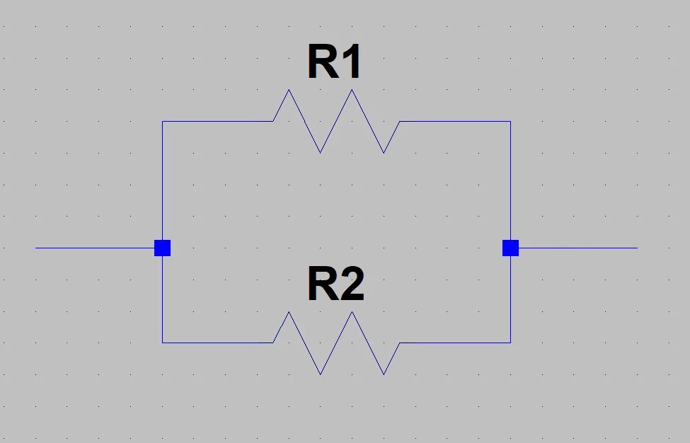
In this article we will deduce how to calculate the resulting resistive value by placing resistors in parallel, i.e. connecting two or more resistors with their interconnected legs. In addition we will use LT Spice to verify these results.
Fig. 1: Example of an arrangement with two generic parallel resistors.
Analyzing figure 1 we can see that the voltage applied to each resistance is the same for all, what will generate a current in each of these, the total current of the source will be the sum of the currents by all the branches of the resistances.
Deduction
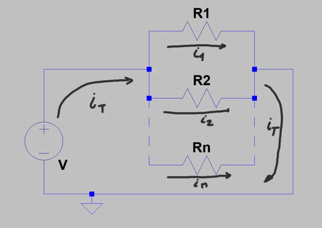
To begin the deduction let’s assume a simple circuit consisting of a V voltage source connected to the parallel resistor array, like the one illustrated in Figure 2.
Fig. 2: Circuit with voltage source and N resistors in parallel. In all resistances the same potential V falls.
On this circuit we are going to apply Kirchoff’s circuit Law for current, which tells us that a node the sum of all the currents that enter the node is equal to the sum of all the currents that leave the node. We consider as node a point that is between the voltage source and the union of all resistances.
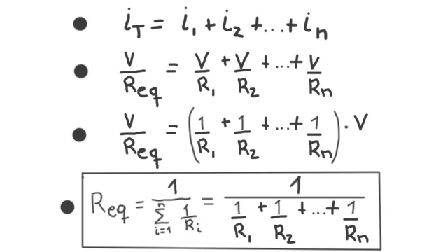
In figure 3, in line 1 I have written what this law tells us considering that we have a finite number of resistances.
On line 2 I place the value of the currents in terms of voltage and resistance according to Ohm’s Law. The next step is to take out the voltage v as a common factor, since all resistors have the same voltage v applied.
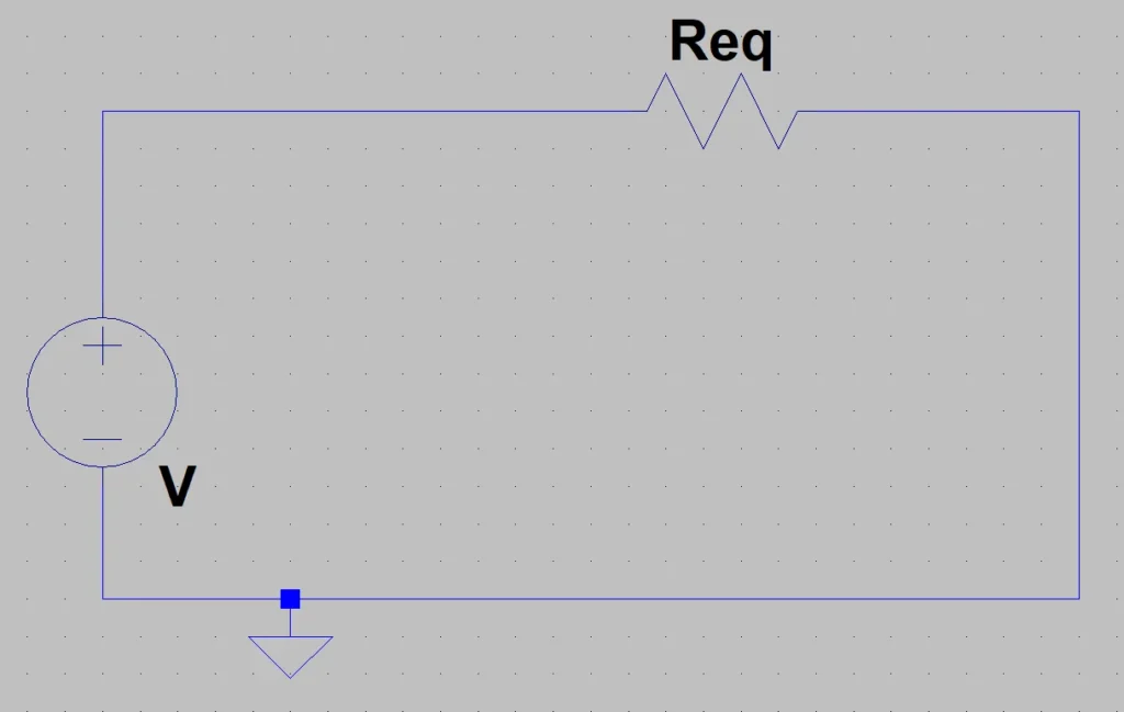
Finally we conclude that what is in parentheses on line 3 is the value of a resistance for an equivalent circuit that instead of having n resistors has only one with this value. In figure 4 we see this equivalent circuit.
Fig. 3: Deduction of the equivalent resistance considering the circuit of the previous figure.
Fig. 4: Same circuit as above but considering that the voltage source is applied to a single resistor with equivalent value.
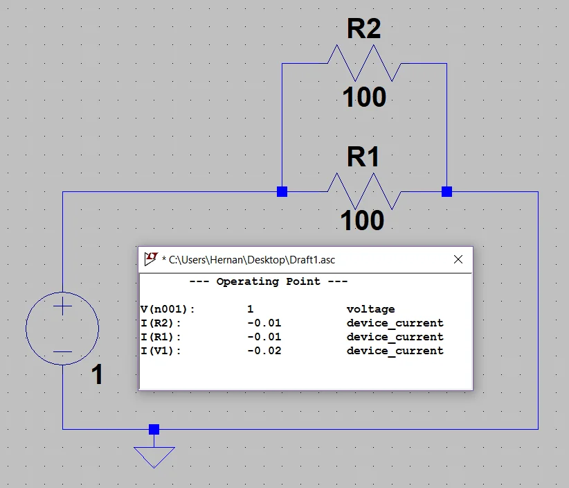
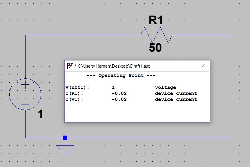
In figure 5 we have simulated a circuit with a voltage source of 1 Volt and two resistances of 100 Ohm connected in parallel, while in figure 6 we have a circuit with the same voltage source but only a resistance with the equivalent resistance value that would be 200 Ohms.
As can be seen in the posters with the result of the simulation, the current circulating through the voltage source is the same in both cases, so we can conclude that these circuits are equivalent.
Fig. 5: Simulation of a circuit with a 1 Volt source and two 100 Ohm resistors in parallel.
Fig. 6: Simulation of a circuit with a source of 1 Volt and a resistance of 200 Ohms.
Conclusion
We have analyzed a circuit with generic parallel resistances and applied the current laws to determine an equivalent expression of resistance.
When we have arrangements of resistances in parallel we know that these have applied the same tension in their extremes, applying Kirchoff’s circuit laws we can deduce an expression for the equivalent resistance.
Finally we have made a simulation to show that we can think of an equivalent circuit grouping the resistances.
Introduction
In this article we will deduce how to calculate the resulting resistive value by placing resistances in series, i.e. connecting two or more chained resistances. We will also use LT Spice to verify these results.
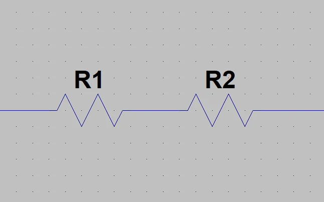
Fig. 1: Example of an arrangement with two generic value resistors in series.
If we think about the physical size of the resistors we realize what the result is going to be. Let’s suppose that we have identical resistances of 100 Ohms that measure 1 cm, if we place two of these resistances one after the other we would have two centimeters of resistive material, then intuitively we can say that two resistances of 100 Ohm in series will result in a resistive value of 200 Ohm.
This reasoning leads us to think that if we have resistors connected in series, their Ohmic value will be added.
Deduction
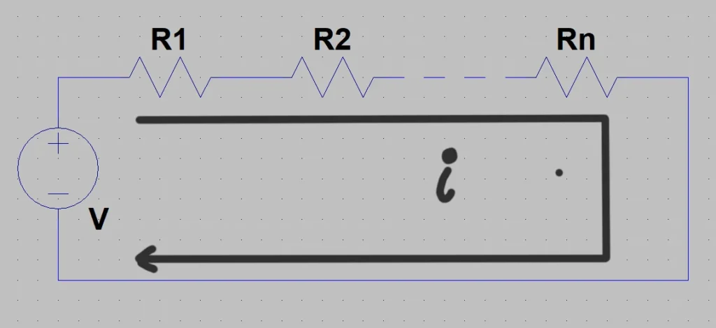
To begin the deduction let’s assume a simple circuit consisting of a V voltage source connected to the array of series resistors, as illustrated in Figure 2.
Fig. 2: Circuit with voltage source and N resistors in series. The same current i circulates through all the resistors.
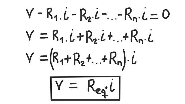
On this circuit we are going to apply Kirchoff’s circuit Law for voltage, which tells us that a closed circuit the sum of all potential drops gives as a result 0.
In figure 3, in line 1 I have written what this law tells us considering that we have a finite number of resistances.
On line 2 I place all the resistors on the right side of the equation. The next step is to take the current i as a common factor, since this same current i circulates through all the resistances.
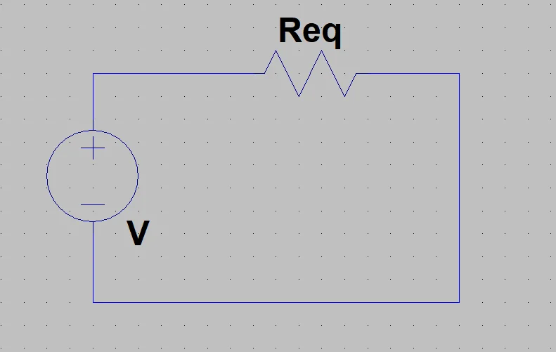
Finally we conclude that what is in parentheses on line 3 is the value of a resistance for an equivalent circuit that instead of having n resistors has only one with this value. In figure 4 we see this equivalent circuit.
Fig. 3: Deduction of the equivalent resistance considering the circuit of the previous figure.
Fig. 4: Same circuit as above but considering that the voltage source is applied to a single resistor with equivalent value.
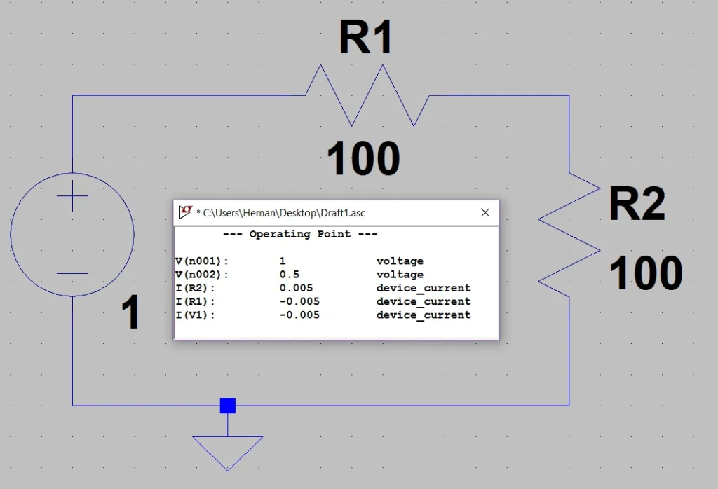
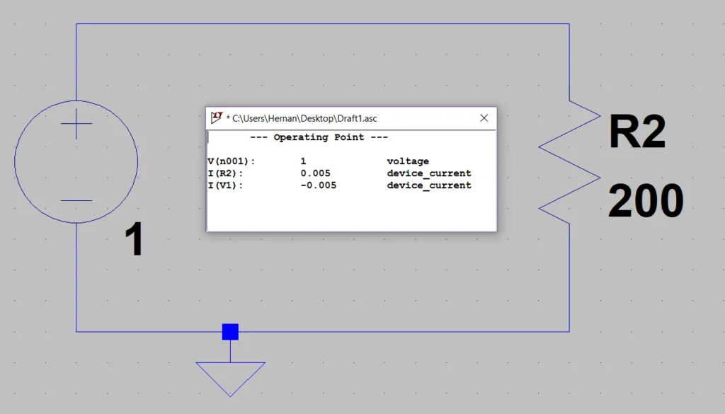
In figure 5 we have simulated a circuit with a voltage source of 1 Volt and two resistances of 100 Ohm connected in series, while in figure 6 we have a circuit with the same voltage source but only a resistance with the equivalent resistance value that would be 200 Ohms.
As can be seen in the posters with the result of the simulation, the current circulating through the voltage source is the same in both cases, so we can conclude that these circuits are equivalent.
Fig. 5: Simulation of a circuit with a 1 Volt source and two 100 Ohm resistors in series.
Fig. 6: Simulation of a circuit with a source of 1 Volt and a resistance of 200 Ohms.
Conclusion
We have intuitively raised what the equivalent resistance value of a series resistor array might be.
When we have arrangements of resistances in series the current that circulates is the same in all, applying Kirchoff’s circuit laws we can deduce an expression for the equivalent resistance.
Finally we have made a simulation to show that we can think of an equivalent circuit grouping the resistances.
Introduction
Without a doubt a useful tool at the time of making tests of operation in the circuits is the Protoboard. In this article we are going to see what it is, sizes, accessories, internal connections and we are going to see examples of incorrect connection and correct connection of elements.
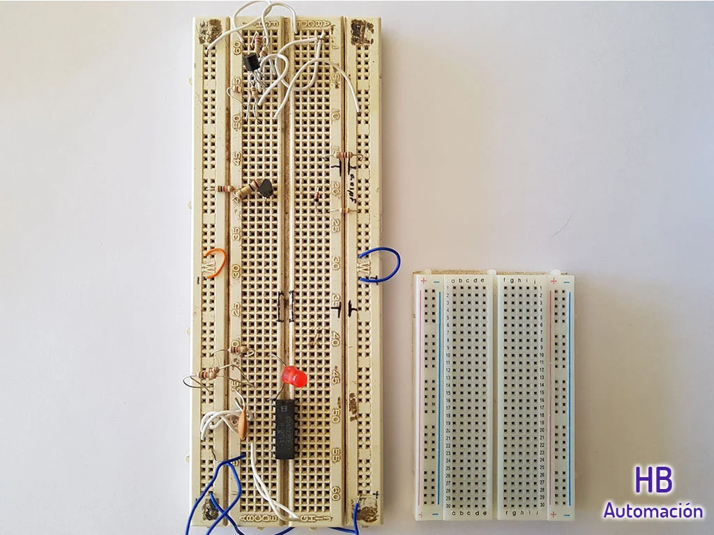
As we see in figure 1 is a plate that has a lot of holes where we can place our components.
Fig. 1: Two examples of protoboards.
Depending on the circuit that we want to implement we may need more than one Protoboard, it is good to know that most have sockets on their sides to fit plates of the same manufacturer.
Fig. 2: The protoboards have sockets that allow one after the other.
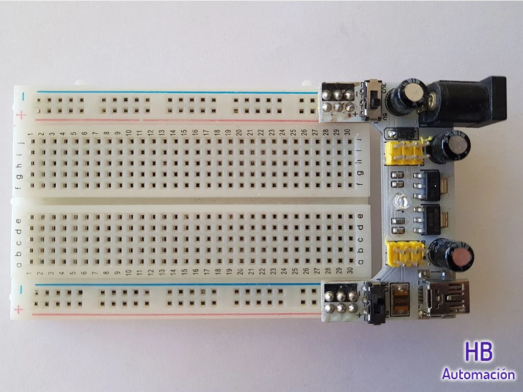
In addition in the market we can find certain accessories that we can use in the protoboard, like cables with male terminals and DC sources.
In the figures 3 and 4 we see an example of these sources that come prepared to place in the protoboard. We can feed it with transformer or with USB cable and train two switches that allow us to choose between 3.2V and 5V.
Fig. 3: Arduino Source ready to be connected to a protoboard.
Fig. 4: This source has a mini USB connection or transformer plug.
Pin Distribution
In figure 5 I have highlighted with colors to show how the electrical bridges under the dot matrix are made.
Fig. 5: Standard bridge of a protoboard.
At both ends of the board we see a red line indicated with a sign “+” and another blue with a sign “-“, these lines are used to provide voltage to our circuits.
In the middle in green color we have 60 lines of 5 points that we can use to make the interconnections of our circuit.
The 5 points on each line are bridged together under the board, which helps us reduce the amount of cables we need.
Another important detail is that we have numbers for the rows and letters for the columns so that we can identify each point of the Protoboard, for example A-1 is the first point at the top right in Figure 5 and J-30 is the last point at the bottom left.
How to connect elements in the Protoboard
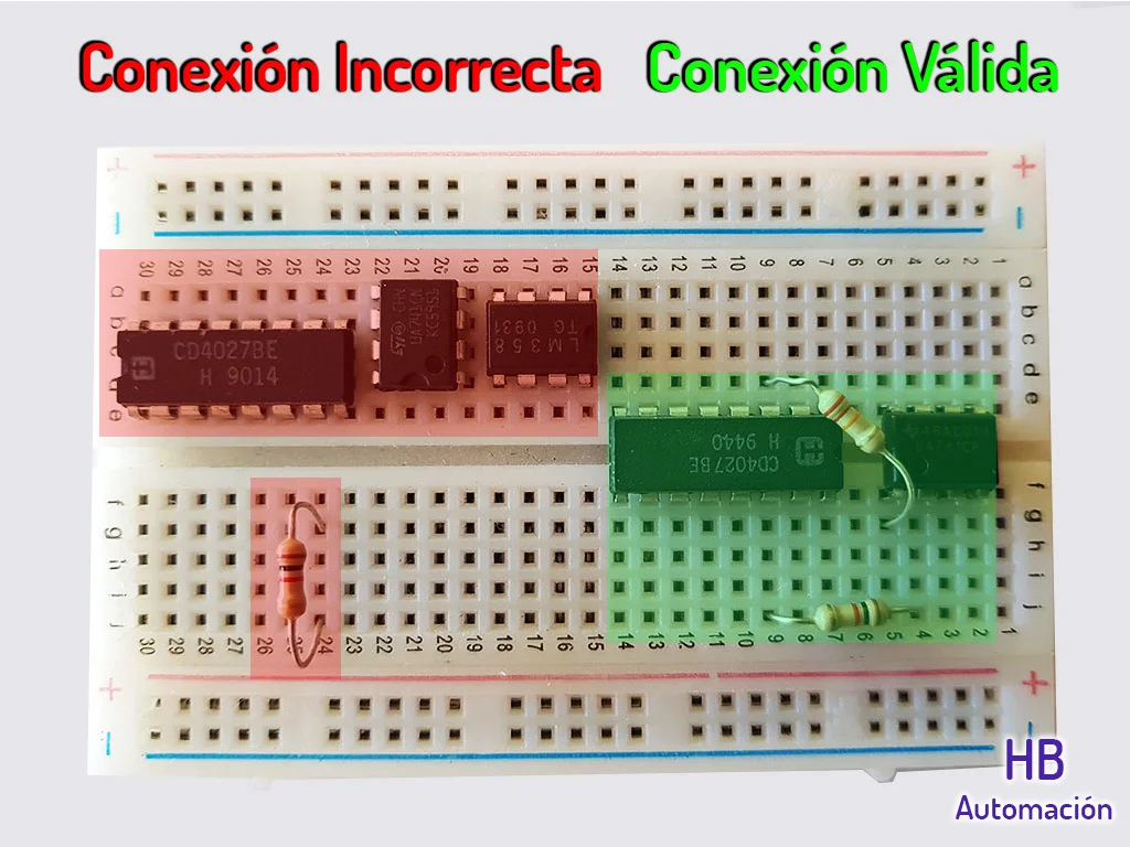
When we have devices with several legs such as transistors or integrated circuits, it is important that we know what the internal distribution of bridges is like, otherwise we can make a mistake in the way they are connected.
In figure 6 we see examples of current and incorrect connections.
Fig. 6: Integrated circuits and resistors in protoboard. Badly connected in red, well connected in green.
For example take the case of the resistance connected at points G-24 and J-24, the 5 points on line 24 from the letter F to J are bridged to each other, so it makes no sense to connect a resistance at two of these points, the current will never flow through it.
Conclusion
The protoboard is a useful tool when testing the operation of our circuits.
Depending on the project, we will need larger or smaller plates, it is good to know that plates of the same type can be fitted using the side skirtings and that there are accessories that can facilitate the supply and connections of the elements.
It is important to know the distribution of the internal bridges of the plate, in this way we will avoid placing the elements badly.
Introduction
In this article we are going to see how to download and install LT Spice software to simulate electrical and electronic circuits. We will also create a simple circuit to test the program.
Download the software
First we will download the installer from the official website, click on the link below:
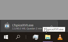
Fig. 1: On the official website we download the program according to our operating system.Fig. 2: The unloading process starts.
Once the download finishes we run it. In my case I got a screen saying that the installation was blocked by the Windows protection system, when I clicked on “More information” the button “Run anyway” appeared.
Fig. 3: Windows blocked the installation, clicking on More Information displays the Run anyway button.
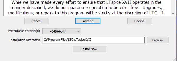
We accept the terms and conditions and choose the installation location. In my case I leave everything by default.
Fig. 4: First we must accept the terms and conditions of the software.
Fig. 5: Choose the installation parameters and click Install Now.
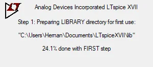
At the end of the installation the program runs automatically, the sign appears in Figure 6 saying that the program is ready to run for the first time.
Fig. 6: At the end of the installation, the software prepares for the first run.
At the end of the process the main window of the program appears, and we are ready to start creating schematics and simulating electrical and electronic circuits.
Fig. 7: This is the main window of the simulation program
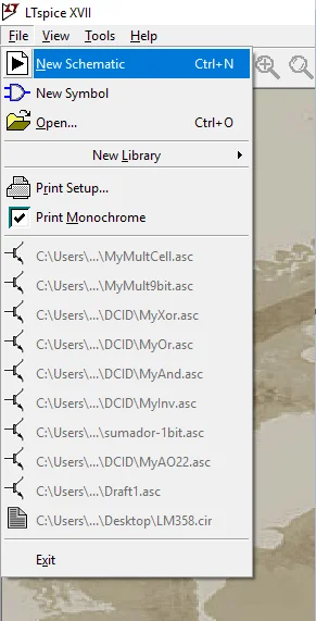
First we go to File > New Schematic, to create a new project, this can be seen in figure 8.
Fig. 8: To start with we create a new schematic.
The workspace appears in gray, here we will begin to build the schematic.
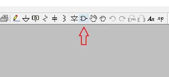
Let’s add elements, click on the AND gate button shown in figure 9.
Fig. 9: Button to add a component to the schematic.
This will display a window in which we can choose the components.
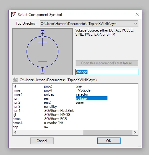
Power Source
To power our circuit we are going to need a voltage source, in the search bar of the components window we write “voltage” and select the generic source that can be seen in figure 10.
Fig. 10: In the window that appears write “Voltage”.
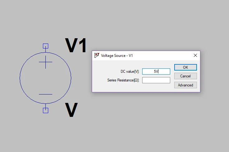
We place it in the workspace and right click on it, this will open a window to enter the parameters of the font, in my case I will use 5 Volts.
The “Advanced” button allows us to define advanced parameters of the source, such as signal type, frequency, period, duration, ascent and descent times, among others. For now we are only going to keep the DC source that comes by default.
Fig. 11: Right click on the voltage source to enter the value.
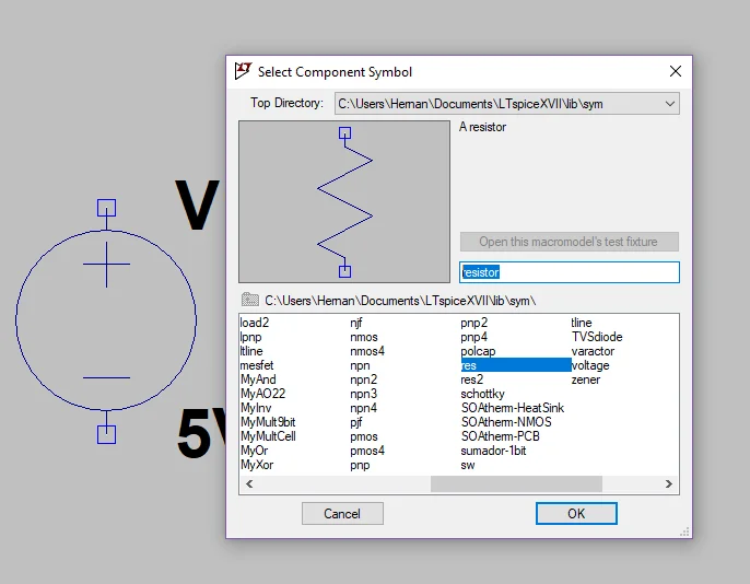
Resistors
Let’s add the resistor, press the button of the AND gate again (figure 9) and this time we write “resistor” in the search bar. Select the generic resistor shown in figure 12.
Fig. 12: Add the “resistor” component to the schematic.
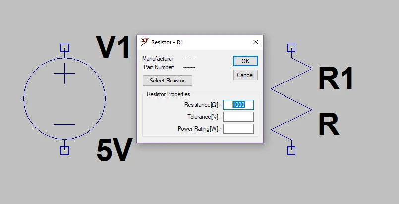
We place it in the workspace and right click on it to enter the parameters.
For now we will only enter a resistance value of 1000 (the standard unit is Ohm, as we see in figure 13 between square brackets to the left of the value 1000).
Fig. 13: Right click on resistance to enter the values.
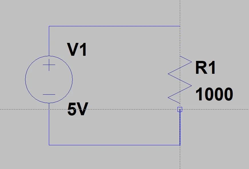
Wiring
When all the elements are in place, let’s make the connections. Click on the pencil button shown in Figure 9 or use the F3 shortcut.
Then we draw the connections between the source and the resistance.
Fig. 14: Use F3 or the menu buttons to make the connections of the elements.
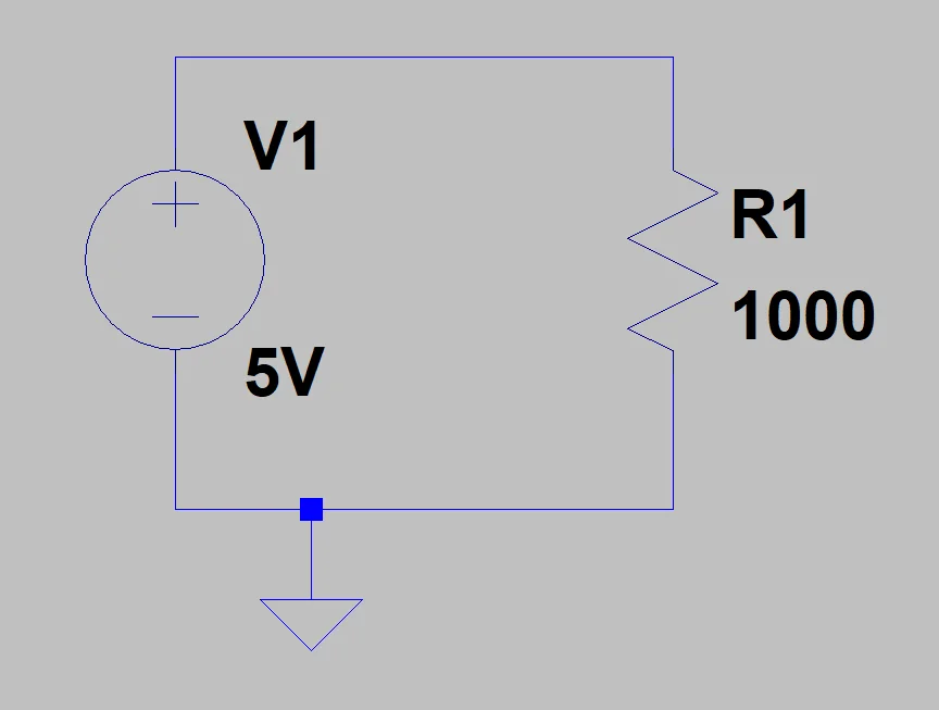
Ground
Finally, in order for the program to perform the calculations, it needs a ground point for reference. Click on the triangular button in figure 9 or with the “G” key.
We place the ground on the cable that is connected to the negative terminal of the source, as shown in figure 15.
Fig. 15: For the schematic to work, a reference ground must be added to the circuit.
Simulation
When we finish the schematic, we go on to configure the simulation parameters.
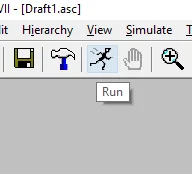
If this is the first time we are going to simulate, click on the Run button shown in figure 16. If this is not the first time, go to the “Simulate” tab and click on “Edit Simulation CMD”.
Fig. 16: Schematic simulation button.
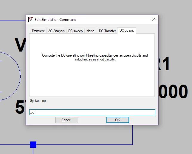
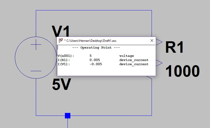
In the Edit Simulation window we are going to choose the last tab called “DC op pnt”, which is shown in figure 17.
Fig. 17: In the simulation configuration window, select the “DC op pnt” tab and click OK.
With this option the program will make a direct current calculation of the circuit, showing the voltages in all the nodes and the currents in all the branches.
Fig. 18: A window appears with the operating values of the DC circuit.
In the window that appears we can see that the current in the resistance is 5 mA, which is condiced with taking the 5 V of the source and dividing them by 1000 Ohms of the resistance, according to the Law of Ohm.
With this we finish the exercise, we are ready to simulate more complex electrical and electronic circuits. In other articles we will talk about how to draw graphs or produce other simulations.
This website uses cookies to improve your experience. We'll assume you're ok with this, but you can opt-out if you wish. Cookie settingsACCEPT
Privacy & Cookies Policy
Privacy Overview
This website uses cookies to improve your experience while you navigate through the website. Out of these cookies, the cookies that are categorized as necessary are stored on your browser as they are as essential for the working of basic functionalities of the website. We also use third-party cookies that help us analyze and understand how you use this website. These cookies will be stored in your browser only with your consent. You also have the option to opt-out of these cookies. But opting out of some of these cookies may have an effect on your browsing experience.
Necessary cookies are absolutely essential for the website to function properly. This category only includes cookies that ensures basic functionalities and security features of the website. These cookies do not store any personal information.